Player Development: The Aging Curve Paradox
A statistical analysis of the uncertainty revolving around development environments
Last week, in my presentation at WHKYHAC, I introduced my new player development framework named DEVe. Separated into 3 sub-models, this framework can be leveraged to evaluate the development trajectories of women’s hockey skaters.
Each sub-model answers a specific question.
Model M1: Will the player retire after this season?
Model M2: If not retiring, in which league will they play next year?
Model M3: How many points will they put up in that league next year?
To learn more about the modelling process for the DEVe project, a link to watch my presentation can be found here.
However, when looking at some individual case studies with the DEVe models, a paradox stood out to some coaches who were providing me feedback before WHKYHAC.
The Paradox
While women’s hockey forwards peak around 26-27 years old, on average, the projected trajectory for some elite players in their early 20s is trending downwards.
Indeed, when looking at the evolution of N-WHKYe with age (for forwards), we note a bell-shaped curve peaking around 26-27 years old. In other words, this means that between the ages of 15 and 27, the projected aging curve for forwards should have an upward trajectory over time.
However, when analyzing the projected aging curves of some elite forwards such as Alina Müller, Josefin Bouveng, Mikyla Grant-Mentis and Petra Nieminen, we observe a downward trending expectation for their development trajectory.
For that reason, inspired by the work of Dom Luszczyszyn (@domluszczyszyn), I incorporated 90% confidence intervals to the projections of model M3. This addition allowed model M3 to consider the uncertainty revolving around development environments by projecting possible ranges of production for years to come.
Interestingly, looking at Dom’s work and more specifically analyzing the projected aging curve for Alex DeBrincat (24 yo), we also note a downward projection trajectory:
To understand why this phenomenon occurs, I went back to analyze some historical numbers.
Retrospective Analysis
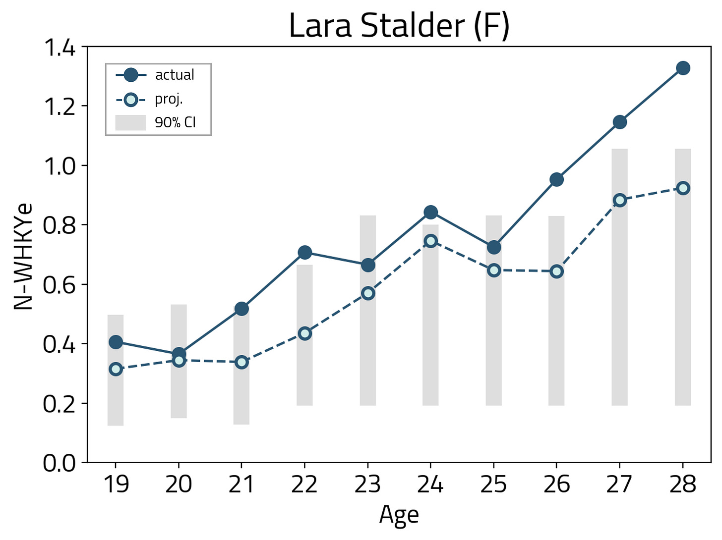
We can do the same exercise of projecting N-WHKYe in time with some historical stats. As a case study, we will take the example of Lara Stalder to analyze retrospective N-WHKYe aging curves. Stalder is a player who consistently put up high production numbers in the last decade.
What’s insightful about Lara Stalder’s retrospective aging curve is the fact that she constantly overachieved her year-over-year projections in the last decade. As such, model M3’s projections were underestimating her ability to continually increase her production rate in different leagues.
Especially when analyzing her last 3 seasons with Brynäs IF in the SDHL, we note that she also put up numbers that were exceeding the upper limit of model M3’s 90% confidence interval.
These insights beg an interesting question regarding the N-WHKYe projections for elite players in the DEVe framework.
And following my presentation, friend of the newsletter, Gilles Dignard (@GillesDignard) had a very interesting thought about this. He asked me if, within the 90% confidence interval, I knew where the median value was compared to my “average” projections.
Investigating his question, which is inherently tied to the idea of probability distributions, could help us answer our initial interrogation on downward trending aging curves for elite players.
Analyzing Deviations
During the validation testing process for model M3, I used mean squared error, among other metrics, as an indicator of model performance. Model M3 actually performed very well in my validation testing, yielding an MSE of 0.006.
The flexible nature of random forest regressors allowed the DEVe framework to explain meaningful variations in our target variable (next year’s N-WHKYe) from the variation of our independent variables (age, league, N-WHKYe and position). Yet, as we described above for elite players, model M3 seemed to be undervaluing future production.
Breaking down the error term by N-WHKYe range can be leveraged to illustrate and further understand the variation of deviations per category of offensive producers.
The animation above shows that as N-WHKYe increases, the more our predictions undervalue future production.
For instance, when looking at all forwards with actual N-WHKYe greater than 0.10, the mean error is 0.047. This means that our predictions are only undervaluing actual future production by 0.047 on average, in this range.
But when only looking at elite forwards (actual N-WHKYe greater than 0.95) the mean error jumps up to 0.475. This time, the mean error informs us that our predictions are significantly undervaluing actual future production, by 0.475 on average.
This confirms our empirical insights gathered with the Stalder case study. The reason why this happens can be put in very simple terms: elite players do elite things. And for that reason, it is “normal” for these elite players to consistently surpass expectations.
However, one aspect of the M3 model which can be improved upon is the confidence interval used as a proxy for estimating uncertainty. Using the above animation as a starting point, enhancing the confidence intervals with distributions could provide us a tool to more precisely evaluate the range of possibilities for coming years.
We will discuss this more in depth, next week, when using a probabilistic approach to uncertainty in the DEVe models.


