
Tactics: A hockey stat that we never talk about (Part 2)
Tactics: A hockey stat that we never talk about (Part 2)
An analysis of how ice time and rest time should be distributed in women's hockey

In our latest post, we analyzed with linear models the benefits of proper rest time for defenders, at even strength. In short, all other things held equal, we concluded that rest time prior to the start of a shift has a positive impact on CF60 (on-ice performance).
However, even if we showed that rest time prior to a shift positively impacts performance, linear models may not be the best way to predict ice-time and rest time, on an individual player basis. This is due to the fact that deployment and rest time (for defenders, in this case) are constrained in a non-linear fashion by many circumstantial factors.
In this second part, we will attempt to simulate deployment patterns for defenders in women’s hockey based on these circumstantial factors. We will once again use data from the latest World Championship and Olympic Games. The goal will be to identify which defenders in international women’s hockey get too little rest and which ones get too much rest between shifts.
To achieve our goal, the first step was to assign a value to defenders based on their overall score (67% of SARAH and 33% of N-WHKYe). This allowed us to determine a ranking of defenders for each team, in a given game.
Model 1: Simulating the passage of time
A hockey game has two inherent states: “play” and “pause”. The “play” state corresponds to the “game segments” as defined by Gilles Dignard (puck drop to whistle). The “pause” state corresponds to the moments during which there is no action (whistle to puck drop).
In order to simulate game time vs pause time, we used the segment length, the score and the strength of play as predictors. For simplicity, we did not try to predict penalties or goals and simply assumed that they would still happen at the times they originally happened in the respective games we simulated.
We built this model as a binary gradient boosting classifier in order to simulate periods on a second-by-second basis, with the following constraints:
an automatic pause of 900 seconds (15 minutes) would occur when game time hit the 1,200 second (20 minute) and 2,400 second (40 minute) marks.
for games that went to overtime, another automatic pause of 900 seconds was added at the 3,600 second mark (60 minutes) and our timer was stopped when the game-winning goal was scored in the real game.
The goal of this model was to obtain a simulated timer for our games which would incorporate both the “play” and the “pause” times. Given that ice time and rest time are inherently related to each other, this first model will later allow us to calculate metrics such as Rest Time above Expected/Shift based on simulated deployment patterns for defenders.
Model 2: Choosing the starters (for the away team)
When thinking about deployment, the first thing that any coach needs to do in a game is to choose his or her starters. That decision depends on factors that may vary from one coach to another. But the universal rule of deployment in hockey (which we will abide by throughout all of our models) is that the home team has the last change.
As such, predicting the starting defense pair for the away team was the initial step in simulating the deployment patterns for defenders. To predict the 2 starting defenders for the away team, we used a weighted randomizer. The weights were based on the most common initial deployment patterns (by defender rank) for each group (A vs B).
As we are only trying to predict defender deployment patterns, we assumed that the starting forwards for both teams were the same as in real life. The same was assumed for every second of “play” time thereafter.
After predicting the starting defense pair for the away team, we then had to predict the starting lineup of the home team. This leads us to talk about the set of models 3.
Models 3: Predicting defender deployment patterns
The starting D pairing for the home team was determined by the set of models 3 as it is similar to most other face-off situations that occur during a game.
Predicting deployment patterns through game simulation is not an easy task. In real life, changes can occur on-the-fly, as well as during pauses. However, for simplicity, we worked around the assumption that changes in our models could only happen during “play” time.
However, this did not mean that our simulated changes could only happen on-the-fly. We were able to separate on-the-fly changes from rotations prior to face-offs by assuming that changes prior to face-offs occurred at the time of the face-off (i.e., at t=0 in a “game segment”).
It was crucial for us to run our models in the right order to abide by the number one rule of deployment described above: the home team has the last change. Therefore, the code for Team 1 (home team) was always ran prior to the code for Team 2 (away team), when simulating games on a second-by-second basis.
Our logic for simulating the deployment patterns can be summarized by the following (simplified) graphic:
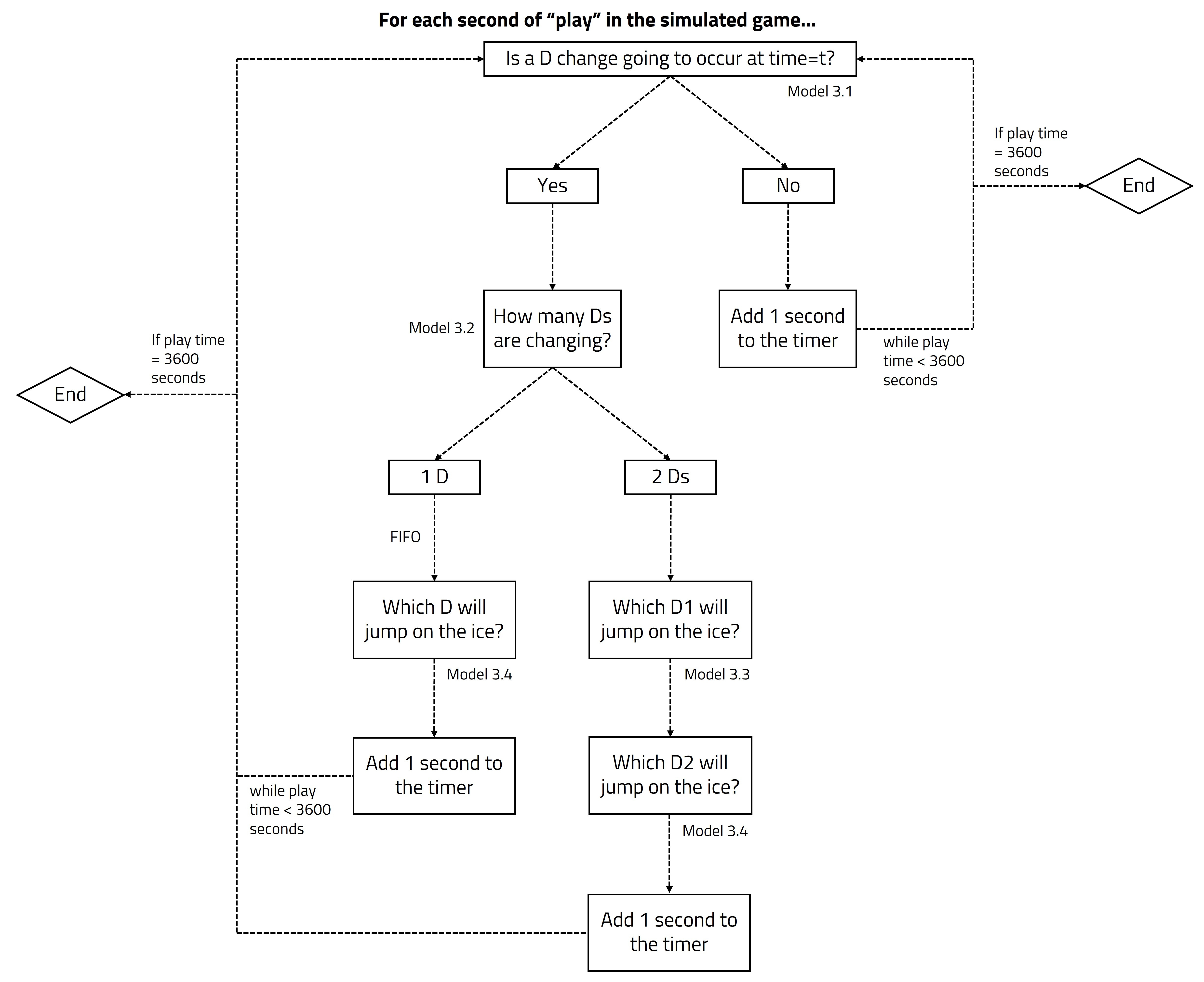
The rationale for simulating defender deployment patterns can be broken down into 4 primary models. Each model answers a specific question that coaches need to ask themselves as part of the deployment decision-making process.
Model 3.1: Should defenders change at time=t?
This is a “yes or no” question. As such, the main goal of this model is to determine whether a defender change is likely to occur at time=t, which always happens in the “play” phase, as explained above.
The three main predictors for this binary gradient boosting classification model are temporal.
First, we have the “segment length”, then we have the “time since the last defender change” and finally the “time since last opposing forward change”.
The “segment length” variable allows our gradient boosting model to recognize face-off situations (where segment length=0). And as it was to be expected, based on the results of model 3.1, changes are more likely to occur at this exact moment in our simulated models.
To put it simply, if the result from model 3.1, for a given second of “play” time, yields a probability of change above 50% for any of the two teams, we then moved on to model 3.2 for that specific team. Otherwise, 1 second second was simply added to the play timer.
Model 3.2: How many defenders should change at time=t?
Most often, this question can be answered by either 1 or 2. The goal of this other binary gradient boosting classifier is to determine whether the shift length for Ds is optimized or not.
As such, to avoid having too many tired Ds on the ice at the same time, this model is built around the same temporal predictors as above. We also added the variable “strength” as a predictor, in model 3.2, to allow our model to identify 4 F, 1 D patterns on the power play for example.
An interesting constraint that our training data adds by itself to model 3.2 is the fact that it is harder to switch 2 defenders on-the-fly as opposed to switching a full D pairing between a whistle and a face-off. And as anecdotal evidence would suggest, we noted in model 3.2 that the full pairing switch option was more likely to occur when the segment length was equal to 0 (i.e., in a face-off situation).
One could argue that we could have used a multi-class gradient boosting model to combine models 3.1 and 3.2 together. However, the 2-model system described above performed better in our (K-Fold) validation tests, with test data from other women’s hockey games with similar level of play.
Models 3.3 and 3.4: Which defender(s) will jump on the ice?
Remember towards the beginning of this article, when we talked about ranking the defenders per team for a given game. This is where that ranking comes into play in our boosting models.
After determining how many defenders will change, models 3.3 and 3.4 determine which defenders are most likely to jump on the ice for the change. For obvious reasons, models 3.3 or 3.4 (when applied at time t) cannot result in predicting either of the 2 Ds that were already present on the ice at time t-1.
In their core essence, models 3.3 and 3.4 are multi-class gradient boosting classifiers built with the goal of determining which defender(s) will jump on the ice based on their strength compared to other Ds in the lineup. The best D of the team is ranked number 1, while the worst D on the team is ranked 6th, 7th or 8th (depending on the number of Ds that the team in question is dressing).
Models 3.3 and 3.4 are built using similar predictors, for the most part:
Quality of Competition (opponents on the ice during the shift, average calculated as 67% of SARAH score & 33% of N-WHKYe)
Quality of Teammates (teammates - forwards - on the ice during the shift, average calculated as 67% of SARAH score & 33% of N-WHKYe)
Group (A or B as categorical variables, excluding Group_B)
Score (-2, -1, 0, 1, 2 as categorical variables, excluding Score_0)
Strength (Even Strength, PP or PK as categorical variables, excluding PK)
When model 3.2 predicts that 2 defenders will switch at time t, model 3.3 is used to determine which defender will jump on the ice first (D1). The rank of D1 is determined with a probabilistic approach: the D rank that has the highest probability in the results of the model (which was not on the ice right before) is deemed to be the new D1.
Model 3.4 is very similar to model 3.3, but instead predicts the second defender (D2) who will jump on the ice. There is one additional predictor to model 3.4, which is the prediction from model 3.3. As such, the rank of D2 is also influenced by the rank of D1 which was predicted right before, when 2 Ds change.
In the case where only 1 D changes, we first look at the 2 defenders on the ice to identify which D has been on for the longest shift. We assume that the defender who has been on for the longest shift is the defender who will change here. In this situation, the D who stays on the ice automatically slides into the D1 slot and we run model 3.4 to determine D2.
Calculating Rest above Expected/Shift
After running the models through all the games, we can combine the results for each defender in order to calculate Rest above Expected/Shift. This metric can be derived as follows:
xRest Time (in a game) = xTotal Time – xTOI
Rest (in a game) = Total Time – TOI
xTotal Time and Total Time respectively represent the total simulated (model 1) and actual game time including both “play” and “pause” sequences.
With these values, we can now calculate Rest above Expected/Shift as:
Rest above Expected/Shift = (Rest – xRest Time)/Number of shifts
Results and Conclusions
When combined, we can get a list of the most overrested (underutilized) and most underrested (overutilized) defenders in the dataset:
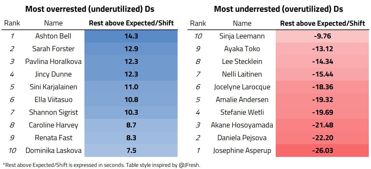
It comes as no surprise to see both Jincy Dunne and Caroline Harvey as part of the most underutilized defenders. Indeed, during the Olympic Games, both defenders saw very little to no ice time, while Team USA’s coach was running a rotation with 5 defenders. This led to some defenders like Lee Stecklein being underrested and overutilized.
Overutilization can have negative impacts on performance as we saw in part 1, where we established a positive relationship between rest time and on-ice performance.
On the contrary, underutilization (i.e., too much rest) could also have negative impacts on performance. While players might be well rested to jump on the ice, coming in cold after a long rest period can have both physical and mental downsides. For the physical aspect, having the right amount of quality rest is more desirable to keep the body reactive and ready to go for the next shift.
From a mental side of things, some players tend to become more nervous when they don’t play much. With nerves, they could start overthinking the game, holding their sticks too tightly or trying to get rid of the puck, with the goal of avoiding mistakes at all costs. By doing this, they seldom add value to their team’s possessions and as a result get even less ice time. And from that point onwards, it can become a vicious circle.
That is why it is crucial for coaches to make players understand and accept their role in a team. Not every defender on a team can play 25 minutes every game. Clearly communicating expectations and ensuring that every defender (and otherwise every player) accepts her role is a key driver of team cohesion. Good team cohesion, in turn, ensures such things as good bench energy and good team spirit, which are crucial for any organization at the highest levels of hockey. But all of this starts with open communication channels between coaches and players (even at the highest levels of hockey).