Player Development: Predicting Development Trajectories with Probabilistic Uncertainty
Bayesian Linear Regression in the context of the DEVe framework

Last week, leveraging Bayes’ rule, we introduced the idea of probabilistic thinking in the context of the DEVe framework. However, we only used Bayesian models to the extent of conjugate priors as they significantly simplify calculations.
We used probabilistic Bayesian models in order to capture the uncertainty revolving around development environments. Taking Alina Müller as an example, we were able to manually calculate the distribution of her projected N-WHKYe thanks to the Normal-Normal conjugacy.
But going beyond our simple case study, we can try to generalize our probabilistic approach with Bayesian Linear Regression.
Methodology
In its essence, Bayesian Linear Regression is similar to “Regular” Linear Regression. As a reminder, here is the formula for “Regular” Linear Regression:

The different terms in this equation can be broken down as follows:
y -> dependent/target variable, the metric we are trying to predict
future N-WHKYe in our case
{X₁, X₂,…, Xₙ} -> predictors/independent variables, the metrics we are using to make our prediction
N-WHKYe, Age and Position in our case
{β₀, β₁, β₂,…, βₙ} -> coefficients, the numbers by which we multiply our predictors to arrive at the target variable
β₀ is the intercept (a constant) and is not associated with any independent variables
ε -> error term, statistical modelling isn’t a perfect science and thus, there must be an error term
the goal of regression is to minimize the error term by fitting the “least squares” regression line based on the data
So, how do we link all this to Bayes’ rule?
In Bayesian frameworks, as we were discussing in our latest post, we set our prior beliefs (“prior”) on what the data looks like and then leverage the actual information we gather (“likelihood”) to adjust our priors.
Moreover, the prior and likelihood follow probability distributions. In that way, we are able to make probabilistic predictions about our target variable.
To run Bayesian Linear Regression models, we need to assign priors to the coefficients associated with each independent variable. In addition, we also assign priors to our intercept and our error term.
In other words, this means that our coefficients, intercept and error term will not be equal to specific numbers in our model. Instead, they will follow a probability distribution. This allows us to link our probabilistic framework to Linear Regression.
The Model
In our Bayesian model, we have 3 predictors: N-WHKYe (current year), Age & Position (as a categorical variable with the forward and defender categories). With this model, we are attempting to predict future N-WHKYe and therefore that is our target variable.
To keep the model simple, we assigned straightforward priors to our coefficients, intercept and error term. For our coefficients and our intercept, we set our priors as normal distributions with mean μ = 0 and standard deviation σ = 1.
The standard deviation of the error term’s prior follows a half cauchy distribution, defined between 0 and +∞, as we want it to be positive.
Given that our data set is large, the simplicity of our priors is acceptable as our Bayesian model will mostly rely on our likelihood to learn and make predictions.
Our model is summarized below:

Results
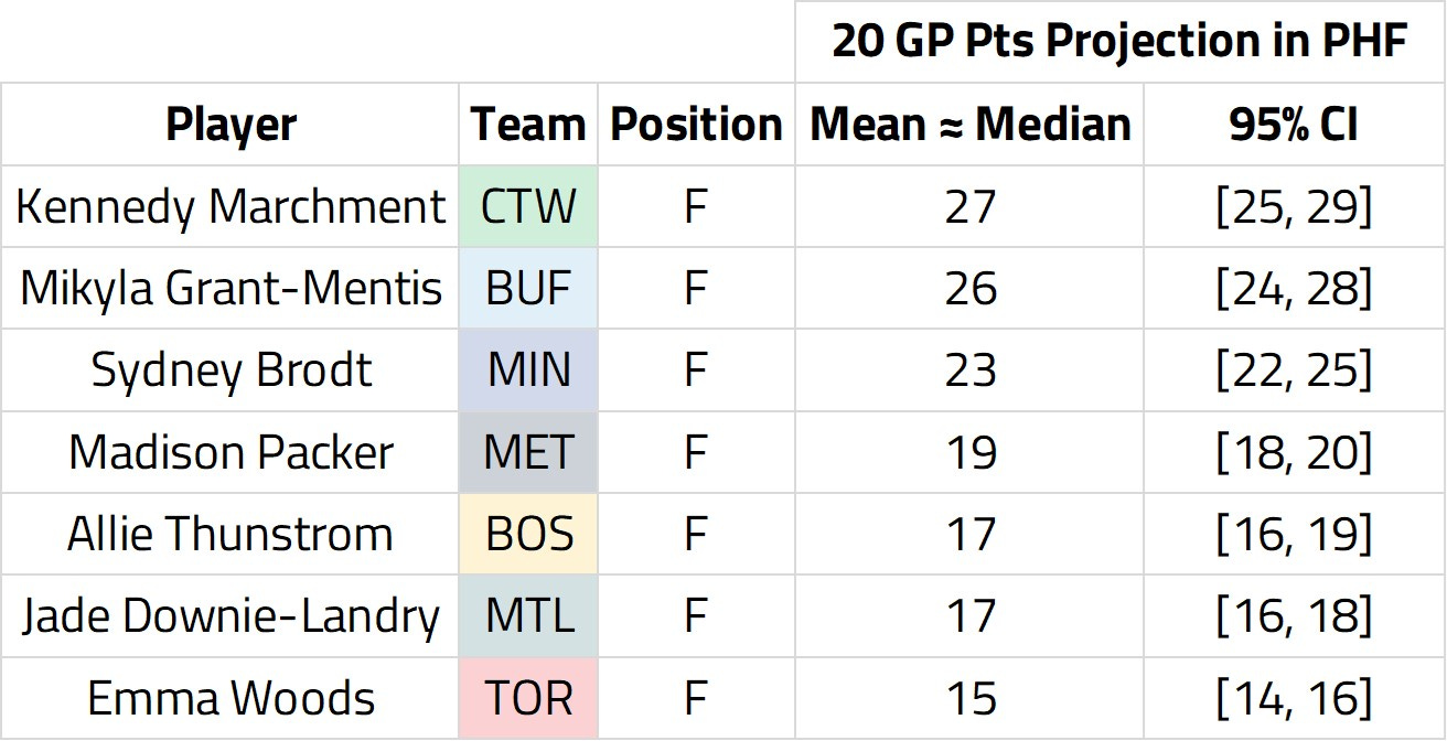
After running our model, we can make probabilistic predictions about the future N-WHKYe of different players.
As the PHF’s free agency is still underway, I decided to make predictions about next year’s N-WHKYe for some key PHF forwards. The list includes:
Kennedy Marchment, Connecticut
Mikyla Grant-Mentis, Buffalo
Sydney Brodt, Minnesota
Madison Packer, Metropolitan
Allie Thunstrom, Boston
Jade Downie-Landry, Montréal
Emma Woods, Toronto

With Bayesian models, instead of getting specific numbers as predictions, we get probability distributions that correspond to a potential range of future N-WHKYe for different players. The mean of these distributions is highlighted in the above chart.
Moreover, we can also leverage credible intervals as part of Bayesian models. 95% credible intervals allow us to say that the “true” value of future N-WHKYe is found in this range with 0.95 probability. Our players’ projected PHF credible intervals can be found below:
Conclusion
Throughout the last month, we’ve explored a framework for analyzing development trajectories of women’s hockey skaters. Beyond the mathematical modelling process, my key takeaways when thinking about aging curves are the following:
It is important to consider the environment in which a player is getting developed in order to correctly assess potential development trajectories for this player.
Developmental trajectories are flexible. They can evolve with time and can vary based on the uncertainty revolving around development environments.
In short, when trying to quantify projected development patterns, it is key to incorporate this uncertainty in one way or another.